First we will load in our data from the GitHub URL.
library(tidyverse)## ── Attaching packages ─────────────────────────────────────── tidyverse 1.3.2 ──
## ✔ ggplot2 3.3.6 ✔ purrr 0.3.4
## ✔ tibble 3.1.8 ✔ dplyr 1.0.9
## ✔ tidyr 1.2.0 ✔ stringr 1.4.1
## ✔ readr 2.1.2 ✔ forcats 0.5.2
## ── Conflicts ────────────────────────────────────────── tidyverse_conflicts() ──
## ✖ dplyr::filter() masks stats::filter()
## ✖ dplyr::lag() masks stats::lag()logs <- read_csv('https://raw.githubusercontent.com/dwillis/NCAAWomensVolleyballData/main/data/ncaa_womens_volleyball_matchstats_2022.csv')## Rows: 6077 Columns: 36
## ── Column specification ────────────────────────────────────────────────────────
## Delimiter: ","
## chr (3): team, opponent, home_away
## dbl (31): team_score, opponent_score, s, kills, errors, total_attacks, hit_...
## lgl (1): result
## date (1): date
##
## ℹ Use `spec()` to retrieve the full column specification for this data.
## ℹ Specify the column types or set `show_col_types = FALSE` to quiet this message.Let’s take a look.
logs## # A tibble: 6,077 × 36
## date team oppon…¹ home_…² result team_…³ oppon…⁴ s kills errors
## <date> <chr> <chr> <chr> <lgl> <dbl> <dbl> <dbl> <dbl> <dbl>
## 1 2022-08-26 A&M-Cor… Nebras… Away NA 0 3 3 20 22
## 2 2022-08-26 A&M-Cor… Pepper… Away NA 0 3 3 36 21
## 3 2022-08-27 A&M-Cor… Tulsa Away NA 2 3 5 75 22
## 4 2022-08-30 A&M-Cor… UTRGV Away NA 2 3 5 78 24
## 5 2022-09-02 A&M-Cor… Sam Ho… Home NA 0 3 3 41 22
## 6 2022-09-03 A&M-Cor… SMU Home NA 0 3 3 41 18
## 7 2022-09-03 A&M-Cor… Indiana Home NA 0 3 3 25 17
## 8 2022-09-06 A&M-Cor… UTRGV Home NA 0 3 3 34 22
## 9 2022-09-09 A&M-Cor… Texas … Away NA 0 3 3 33 20
## 10 2022-09-10 A&M-Cor… Rice Away NA 0 3 3 36 21
## # … with 6,067 more rows, 26 more variables: total_attacks <dbl>,
## # hit_pct <dbl>, assists <dbl>, aces <dbl>, s_err <dbl>, digs <dbl>,
## # r_err <dbl>, block_solos <dbl>, block_assists <dbl>, b_err <dbl>,
## # pts <dbl>, bhe <dbl>, defensive_kills <dbl>, defensive_errors <dbl>,
## # defensive_total_attacks <dbl>, defensive_hit_pct <dbl>,
## # defensive_assists <dbl>, defensive_aces <dbl>, defensive_s_err <dbl>,
## # defensive_digs <dbl>, defensive_r_err <dbl>, defensive_block_solos <dbl>, …We want to group these game logs by team and then summarize them by adding up each game’s blocks, kills, and aces. We use a special formula to calculate points scored from blocks. We’ll store this in a new dataframe called totals.
totals <- logs %>% group_by(team) %>%
  summarize(total_kills = sum(kills), total_blocks = sum(block_solos) + (round(sum(block_assists)/2)), total_aces = sum(aces))
totals
## # A tibble: 345 × 4
## team total_kills total_blocks total_aces
## <chr> <dbl> <dbl> <dbl>
## 1 A&M-Corpus Christi Islanders 991 111 96
## 2 Abilene Christian Wildcats 804 93 93
## 3 Air Force Falcons 871 175 120
## 4 Akron Zips 797 111 77
## 5 Alabama A&M Bulldogs 646 108 89
## 6 Alabama Crimson Tide 879 147 138
## 7 Alabama St. Lady Hornets 831 128 130
## 8 Alcorn Lady Braves 480 80 66
## 9 American Eagles 910 159 115
## 10 App State Mountaineers 818 151 108
## # … with 335 more rowsIf we filter by team, we can find Maryland and make a variable that has the season totals.
totals %>% filter(team == "Maryland Terrapins, Terps")## # A tibble: 1 × 4
## team total_kills total_blocks total_aces
## <chr> <dbl> <dbl> <dbl>
## 1 Maryland Terrapins, Terps 767 228 133md <- c("Kills" = 767, "Blocks" = 228, "Aces" = 133)Let’s try and plot this on a waffle chart. We need to load in our waffle library and format the plot so we can understand it.
library(waffle)
waffle(
md,
rows = 10,
title="Maryland Volleyball's Offense",
xlab="1 square = 1 point",
colors = c("red", "orange", "yellow")
)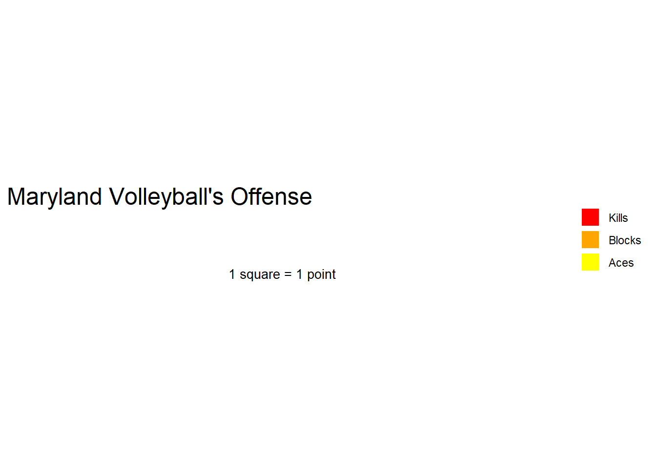 Well… the squares are too small. What if we increase the scale of each square and add some more default rows?
md <- md/2
waffle(
md,
rows = 14,
title="Maryland Volleyball's Offense",
xlab="1 square = 2 points",
colors = c("red", "orange", "yellow")
)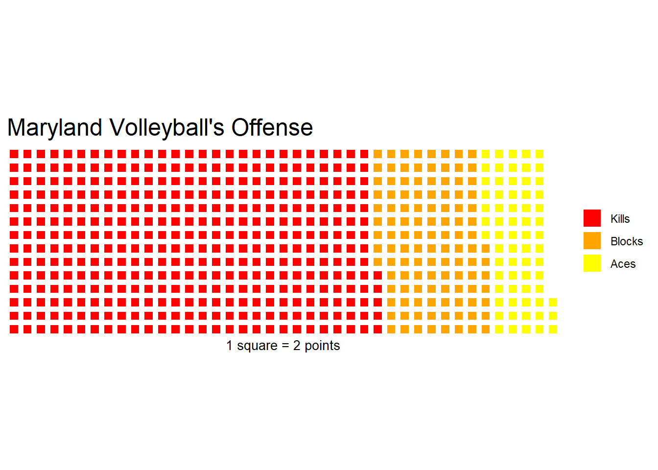 Better. But now we should compare to another team and see how the Terps stack up. I picked Michigan because that’s where my dad went.
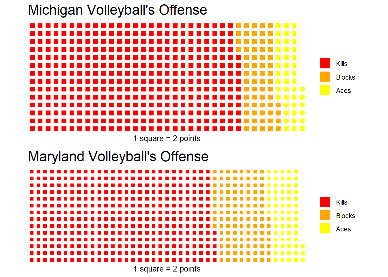
totals %>% filter(team == "Michigan Wolverines")## # A tibble: 1 × 4
## team total_kills total_blocks total_aces
## <chr> <dbl> <dbl> <dbl>
## 1 Michigan Wolverines 748 128 88We’ll make another variable for their totals and divide by two to match the same scale as before. If we use the iron function we can plot the two teams side by side.
mich <- c("Kills" = 748, "Blocks" = 128, "Aces" = 88)
mich <- mich/2
iron(
waffle(
        mich,
        rows = 14,
        title="Michigan Volleyball's Offense",
        xlab="1 square = 2 points",
        colors = c("red", "orange", "yellow")
),
waffle(
        md,
        rows = 14,
        title="Maryland Volleyball's Offense",
        xlab="1 square = 2 points",
        colors = c("red", "orange", "yellow")
)
)
Almost done. We need to make sure each square is the same size across teams so that we can compare. Michigan scored less points, so they need to be padded with whitespace. We’ll take the difference of the two vectors and add it to Michigan’s. After we divide by 2, this should fill in the difference with white squares instead of enlarging the squares.
mich <- c("Kills" = 748, "Blocks" = 128, "Aces" = 88, sum(md - mich)*2)
mich <- mich/2
iron(
waffle(
mich,
rows = 14,
title="Michigan Volleyball's Offense",
xlab="1 square = 2 points",
colors = c("red", "orange", "yellow", "white")
),
waffle(
md,
rows = 14,
title="Maryland Volleyball's Offense",
xlab="1 square = 2 points",
colors = c("red", "orange", "yellow")
)
)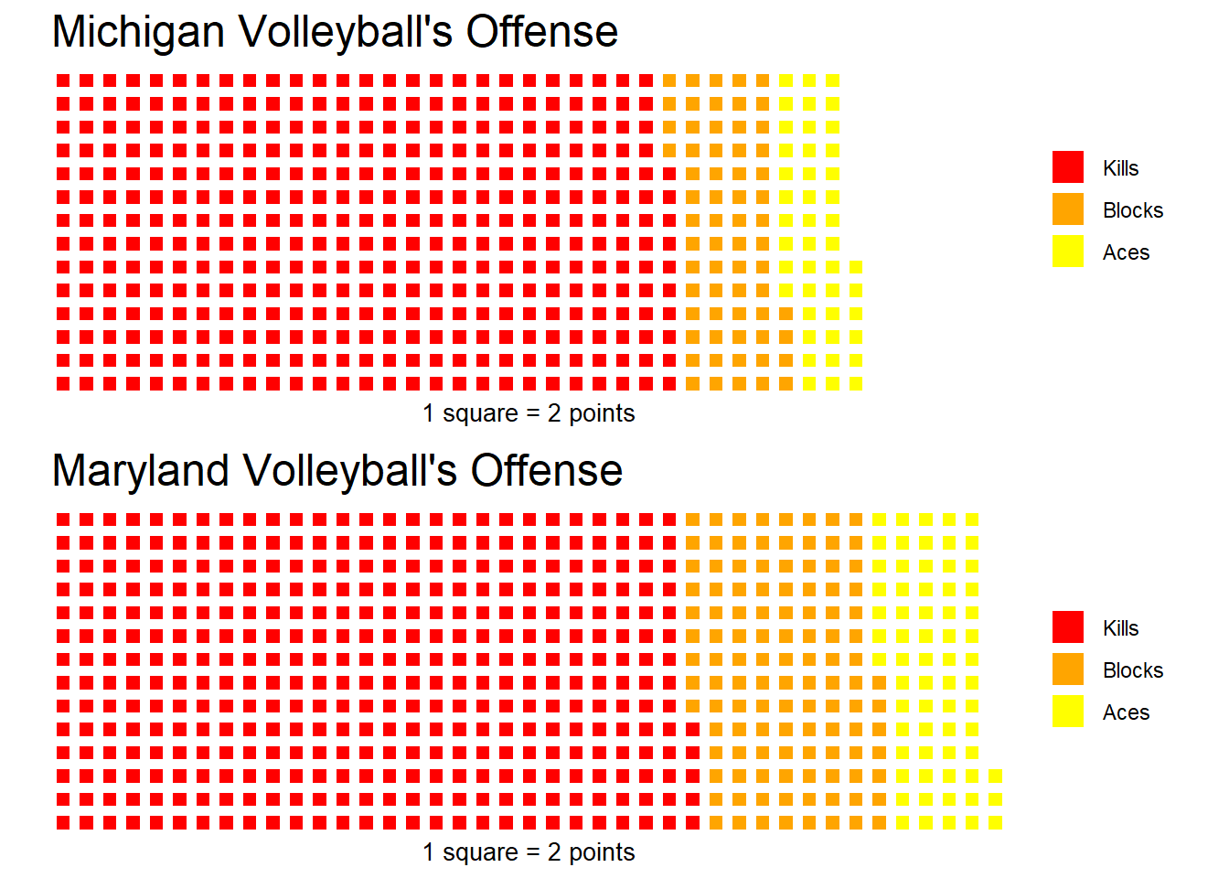 Cool! Maryland has scored more points than Michigan. Both teams get about the same amount of points from kills though. Maryland only has 8 more. Maryland gets a lot more blocks and a handful more aces though. This is what really creates the gap between the two teams’ totals.